Linear, Logistic, and Cox Regression

What regression actually does

A regression model estimates how an outcome tends to change as one or more predictors change, while holding every other variable in the model constant. Feed it a dataset of patients along with the exposure being studied and whatever other variables might matter, and it returns a single number for each predictor describing its independent relationship with the outcome.

That single number is what makes regression so useful, and so easy to misuse. It looks like a clean, isolated answer. Understanding what it actually represents, and what it does not, starts with a phrase this series has already used more than once.

Why adjusted for almost always means regression

Earlier in this series, when discussing confounding, a study reporting an outcome as adjusted for age, sex, and comorbidities was mentioned without fully explaining how that adjustment actually happens. Regression is how. Building a model that includes the exposure of interest alongside those other variables, the coefficient on the exposure becomes an estimate of its relationship with the outcome after mathematically accounting for the others.

This is also why regression cannot rescue a study from unmeasured confounding, a limitation covered in that earlier post. A model can only adjust for a variable that was actually collected and included. Everything else, however important, is invisible to it.

Take a study asking whether a new anticoagulant reduces stroke risk compared with standard therapy, adjusted for age, kidney function, and prior stroke history. Building a single regression model with the anticoagulant, age, kidney function, and prior stroke history all included together, the coefficient attached to the anticoagulant term is the very adjusted effect the study reports as its headline result. The other three coefficients in that same model, the independent relationships of age, kidney function, and prior stroke history with the outcome, exist in the output too, most studies simply do not bother reporting them because nobody asked.

Matching the model to the outcome

Which type of regression to use is mostly determined by one question: what kind of outcome are you trying to explain.

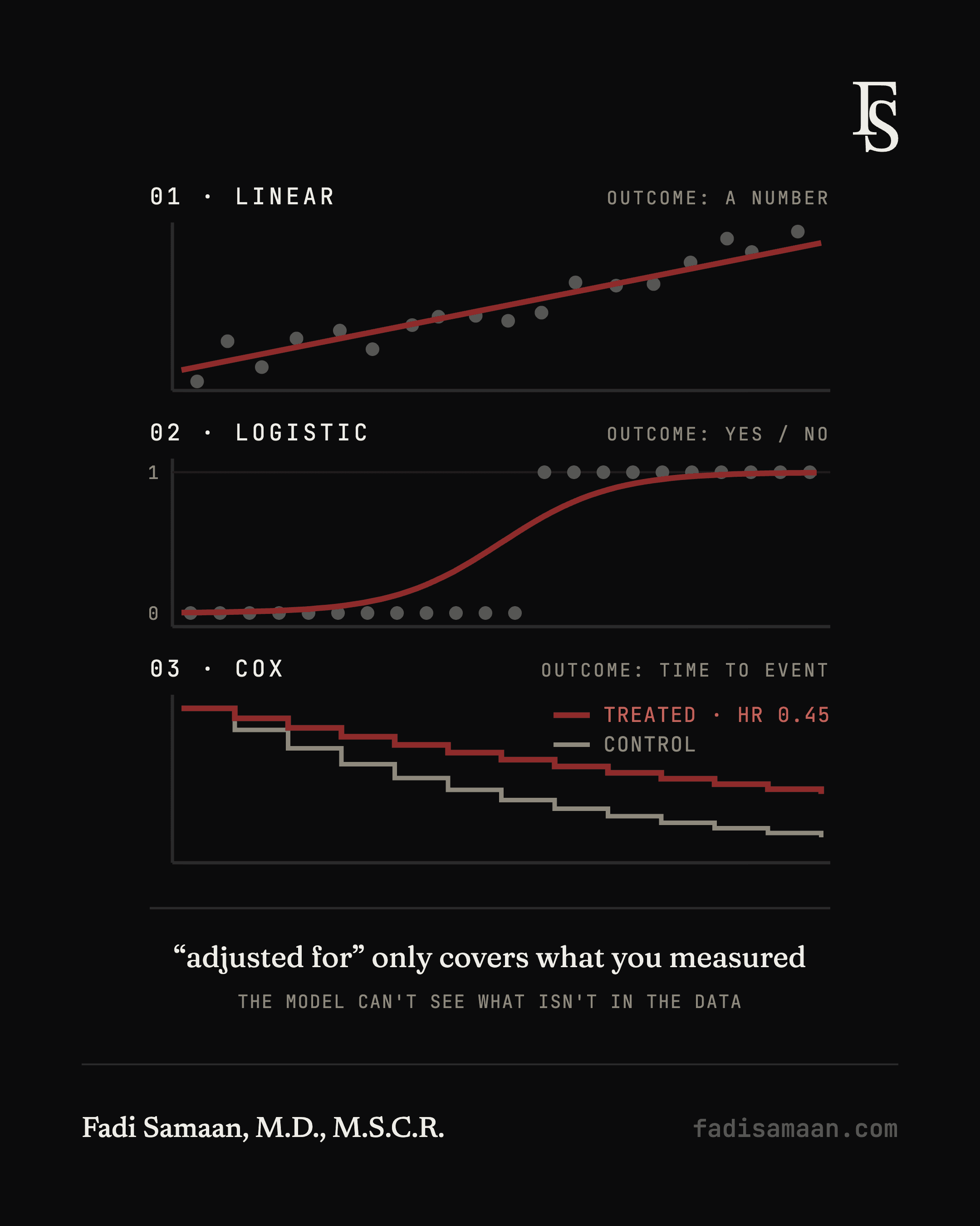
Linear regression is used when the outcome is a continuous number, blood pressure, weight, a lab value. Its coefficient represents the average change in that outcome for every one unit increase in a predictor, holding the other predictors constant. A model relating systolic blood pressure to daily sodium intake, adjusted for age, weight, and kidney function, might report a coefficient of 0.4, meaning every additional gram of sodium per day is associated with a 0.4 point rise in systolic blood pressure, independent of those other three variables.

Logistic regression is used when the outcome is binary, a disease present or absent, an event that either happened or did not. Its raw coefficient is on a less intuitive scale, so it is almost always exponentiated before being reported, turning it into an odds ratio, the same quantity introduced in the relative risk and odds ratio blog, describing how the odds of the outcome shift with each predictor. A logistic model relating smoking status to lung cancer, adjusted for age and occupational exposure, might report an odds ratio of 3 for smoking, meaning smokers have three times the odds of developing lung cancer compared with nonsmokers who otherwise match on age and occupational exposure.

Cox proportional hazards regression is used when the outcome is time to an event, how long until death, relapse, or discharge, rather than simply whether the event happened. It is built to handle censoring, patients who leave a study, or the study ends, before their event occurs, still contributing the time they were observed without being treated as if they never had the outcome. Its coefficient exponentiates into a hazard ratio, describing how quickly the event tends to occur in one group relative to another. A Cox model comparing two chemotherapy regimens might report a hazard ratio of 0.7 for the newer regimen, meaning patients on it experience relapse at roughly 70 percent the rate of patients on the standard regimen at any given point during follow up.

Picking the right one is rarely a judgment call. A continuous lab value calls for linear regression, a yes or no diagnosis calls for logistic regression, and a study tracking time until something happens calls for a Cox model. Using the wrong type distorts the coefficient, whatever else about the analysis is done correctly.

What could go wrong

A regression coefficient can look precise and still be misleading, for reasons that have nothing to do with which type of model was chosen.

Overfitting happens when a model includes too many predictors relative to the number of patients, or more precisely the number of events, in the dataset. With enough variables, a model can fit the noise in that specific dataset rather than a genuine underlying pattern, producing results that look impressive on the data it was built on and fall apart on new patients, the same optimism problem raised earlier when discussing AUC measured on a model’s own training data. A commonly cited rule of thumb for logistic and Cox models is roughly ten to twenty events per predictor included, fewer than that and the risk of overfitting climbs quickly, regardless of how large the overall dataset looks on paper.

Multicollinearity occurs when two or more predictors in a model are highly correlated with each other, height and body surface area, for instance. The model struggles to separate their individual effects, and their coefficients can become unstable, sometimes even flipping sign or losing statistical significance entirely, without the model’s overall predictions being wrong at all. The individual coefficients simply stop being reliably interpretable, even while the model as a whole still performs reasonably well.

Extrapolation is applying a model’s results outside the range of data it was actually built on. A model trained on patients between 40 and 70 years old says nothing reliable about a 25 year old or a 90 year old, even though the equation will happily produce a number for either one if asked. The relationship a model describes was only ever verified within the range of data that went into building it.

The most important pitfall is the simplest to state and the easiest to forget: a coefficient is an association, not proof of causation. A regression model can only adjust for variables that were actually measured and included. An exposure’s coefficient can look meaningfully independent of every variable in the model and still be confounded by something nobody thought to collect, exactly the residual confounding problem from earlier in this series, dressed up in a more sophisticated looking number.

A regression coefficient is only as trustworthy as the variables included in the model and the range of data it was built on.

Key Takeaways

• Regression estimates how an outcome changes with a predictor while holding other included variables constant, which is literally what a study means by adjusted for.

• Model choice depends on the outcome: linear regression for a continuous outcome, logistic regression for a binary outcome, and Cox regression for a time to event outcome with censoring.

• Logistic regression coefficients exponentiate into odds ratios; Cox regression coefficients exponentiate into hazard ratios.

• Too many predictors for too few patients causes overfitting, a model that performs well on its own data and poorly on new patients.

• Highly correlated predictors, multicollinearity, can make individual coefficients unstable even when the model’s overall predictions remain sound.

• A regression coefficient reflects association within the variables the model actually included, not proof of causation, and cannot adjust for a confounder nobody measured.

Up Next:

Next, we will step back from a single study’s model to combining several studies at once with meta-analysis and forest plots, and see how one overall estimate gets built out of many separate results.